Data Generator

The Data Generator is a tool to generate timeseries data which adheres to a statistical model described by a schema.

It can be used for both populating a database as well as having a way to continuously insert timeseries data.

Installation

PyPI package

The Time Series Data Generator tsperf package and can be installed using pip.

pip install tsperf

OCI image

Another way to run the Data Generator is to use the OCI image ghcr.io/crate/tsperf.

• Adapt one of the example docker-compose files in the example folder.

• Start (e.g. CrateDB example) with docker-compose -f examples/basic-cratedb.yml up.

Configure TSDG using environment variables. See also example use cases.

Usage

• Look at the default configuration of the Data Generator by executing tsperf write --help in a terminal.

• Run the Data Generator with the desired configuration values by executing tsperf write in a terminal.

To look at example configurations navigate to the example folder. Each environment variable can be overwritten by using the corresponding command line argument.

Supported Databases

Currently, 7 databases are supported.

• CrateDB

• InfluxDB V2

• Microsoft SQL Server

• MongoDB

• PostgreSQL

• TimescaleDB

• Timestream

Databases can be run either local or in the Cloud as both use cases are supported. Support for additional databases depends on the demand for it.

The following chapters give an overview over the specific implementation for the different databases.

CrateDB

For CrateDB the crate library is used. In order to connect to CrateDB, the following environment variables must be set:

• ADDRESS: hostname including port e.g. localhost:4200

• USERNAME: CrateDB username.

• PASSWORD: password for CrateDB user.

Table Setup

A table gets it’s name either from the provided schema or from the environment variable TABLE

A table for CrateDB has three columns:

• ts: column containing a timestamp (occurrence of the payload)

• g_ts_'interval': column containing the ts value truncated to the value set with PARTITION. It is used to partition the table and generated by the DB.

• payload: column containing the the values, is of type OBJECT Dynamic. The concrete subcolumns are defined by the provided schema.

Additional table configuration:

• with SHARDS the amount of shards for the table can be configured

• with REPLICAS the amount of replicas for the table can be configured

Insert

Insert is done using the unnest function of CrateDB.

Notes

• All columns and sub-columns are automatically indexed

• Using an object column makes it possible to insert the values for multiple schemas into a single table (similar to a schema-less approach of a NO-SQL database).

• Using unnest for the insert makes it possible to take the generated values without modification and insert them directly into the table.

InfluxDB

For InfluxDB the influx-client library is used as the Data Generator only supports InfluxDB V2. To connect to InfluxDB, the following environment variables must be set:

• ADDRESS: Database address. Either a DSN URI, or hostname:port.

• TOKEN: InfluxDB Read/Write token

• ORG: InfluxDB organization

Bucket Setup

A bucket gets it’s name either from the provided schema or from the environment variable TABLE

If a bucket with the same name already exists on the given host this bucket is used to insert data otherwise a new bucket is created without retention rules (data is saved indefinitely)

Insert

Insert into InfluxDB is done using the Point type from the influxdb_client.client.write.api. All tags from the schema are added to Point.tag (InfluxDB creates indices for tags). Measurements are saved to Point.field. The timestamp is added to Point.time. Multiple Points are then inserted in a batch.

Notes

• All tags are automatically indexed

• Insert of multiple schemas into a single bucket is possible due to InfluxDB being a NoSQL database.

• When using InfluxDB V2 with a usage-based plan insert is limited to 300MB/5m, this is about 15.000 data points per second. Excess data is dropped by InfluxDB and the client is not informed.

Microsoft SQL Server

For Microsoft SQL Server the pyodcb library is used. If the Data Generator is run via pip install please ensure that pyodbc is properly installed on your system.

To connect to Microsoft SQL Server, the following environment variables must be set:

• ADDRESS: the host where Microsoft SQL Server is running in this format

• USERNAME: Database user

• PASSWORD: Password of the database user

• DATABASE: the database name to connect to or create

Table Setup

A table gets it’s name from the provided schema

A table for Microsoft SQL Server consists of the following columns:

• ts: column containing a timestamp (occurrence of the payload)

• a column for each entry in tags and fields.

  • tags are of type INTEGER when using numbers and of type TEXT when using list notation

  • fields are of the type defined in the schema

If a table or database with the same name already exists it will be used by the data generator

Insert

The insert is done using the executemany function

MongoDB

For MongoDB the MongoClient library is used.

To connect to MongoDB, the following environment variables must be set:

• ADDRESS: hostname (can include port if not standard MongoDB port is used)

• USERNAME: username of TimescaleDB user

• PASSWORD: password of TimescaleDB user

• DATABASE: The name of the MongoDB database that will be used

Collection Setup

A collection gets it’s name from the provided schema.

A document in the collection consists of the following elements:

• measurement: same as the collection name

• date: the timestamp of the measurement in datetime format

• tags: tags that were defined in the schema

• fields: fields that were defined in the schema

Insert

Insert is done using the insert_many function of the collection to insert documents in batches.

Notes

• MongoDB only creates a default index other indices have to be created manually.

• Insert of multiple schemas into a single collection is possible but it’s advised to use different collections for each schema (same database is fine).

PostgreSQL

For PostgreSQL the psycopg2 library is used.

To connect to PostgreSQL, the following environment variables must be set:

• ADDRESS: hostname

• USERNAME: username of TimescaleDB user

• PASSWORD: password of TimescaleDB user

• DATABASE: the database name with which to connect

Table Setup

A table gets it’s name either from the provided schema or from the environment variable TABLE.

A table for PostgreSQL consists of the following columns:

• ts: column containing a timestamp (occurrence of the payload)

• ts_'interval': column containing the ts value truncated to the value set with PARTITION.

• a column for each entry in tags and fields.

  • tags are of type INTEGER when using numbers and of type TEXT when using list notation

  • fields are of the type defined in the schema

If a table with the same name already exists which doesn’t have the expected structure the data-generator will fail when inserting values.

Insert

Insert is done in batches.

Notes

• No index is created, to query data indices must be created manually.

• Insert of multiple schemas into a single table is not possible as the table schema is only created once.

TimescaleDB

For TimescaleDB the psycopg2 library is used. As psycopg2 does not have the best insert performance for TimescaleDB (see here), to insert a lot of data points, it is advised to split IDs over multiple data-generator instances.

Note: starting with version 0.1.3 TimescaleDB uses the pgcopy library by default to enhance insert performance for single clients. To override the default setting you can set TIMESCALE_COPY to False.

To connect to TimescaleDB, the following environment variables must be set:

• ADDRESS: Database address

• USERNAME: username of TimescaleDB user

• PASSWORD: password of TimescaleDB user

• DATABASE: the database name with which to connect

Table Setup

A table gets it’s name either from the provided schema or from the environment variable TABLE

A table for TimescaleDB consists of the following columns:

• ts: column containing a timestamp (occurrence of the payload)

• ts_'interval': column containing the ts value truncated to the value set with PARTITION.

• a column for each entry in tags and fields.

  • tags are of type INTEGER when using numbers and of type TEXT when using list notation

  • fields are of the type defined in the schema

If a table with the same name already exists which doesn’t have the expected structure the data-generator will fail when inserting values.

Using this table a TimescaleDB Hypertable is created partitioned by the ts and ts_'interval' column

Insert

Insert is done in batches.

Notes

• No index is created, to query data indices must be created manually.

• Insert of multiple schemas into a single table is not possible as the table schema is only created once.

• psycopg2 does not have the best insert performance for TimescaleDB (see here) to insert a lot of data points, it is advised to split IDs over multiple data-generator instances.

• TimescaleDB can be used with distributed hypertables. To test the data generator on hypertables, the TIMESCALE_DISTRIBUTED environment variable must be set to True.

Timestream

For AWS Timestream the boto3 library is used.

To connect to AWS Timestream, the following environment variables must be set:

• AWS_ACCESS_KEY_ID: AWS Access Key ID

• AWS_SECRET_ACCESS_KEY: AWS Secret Access Key

• AWS_REGION_NAME: AWS Region

• DATABASE: the database name to connect to or create

Table Setup

A table gets it’s name from the provided schema

A table for AWS Timestream consists of the following columns:

• A column for each tag in the provided schema

• All columns necessary for the AWS Timestream datamodel:

If a table or database with the same name already exists it will be used by the data generator

Insert

The insert is done according to the optimized write documentation. Values are grouped by their tags and inserted in batches. As AWS Timestream has a default limit of 100 values per batch, the batch is limited to have a maximum size of 100.

Notes

Tests show that about 600 values per second can be inserted by a single data generator instance. So the data schema has to be adjusted accordingly to not be slower than the settings require.

For example, having 600 sensors with each 2 fields, and each should write a single value each second, would require 1200 values/s of insert speed. For satisfying this scenario, at least 2 data generator instance would be needed.

Configuration

The Data Generator is mostly configured by setting environment variables or command line arguments. Start with -h for more information. This chapter lists all available environment variables, and explains their use in the Data Generator.

Environment Variables

Configure the behaviour of the data generator using environment variables.

CONCURRENCY

Type:

Integer

Value:

A positive number.

Default:

1

The Data Generator will split the insert into as many threads as this variable indicates.

ID_START

Type:

Integer

Value:

A positive number. Must be smaller than ID_END.

Default:

1

The Data Generator will create (ID_END + 1) - ID_START channels.

ID_END

Type:

Integer

Value:

A positive number. Must be greater than ID_START.

Default:

500

The Data Generator will create (ID_END + 1) - ID_START channels.

INGEST_MODE

Type:

Boolean

Value:

False or True

Default:

True

INGEST_MODE False

When INGEST_MODE is set to False the Data Generator goes into “steady load”-mode. This means for all channels controlled by the Data Generator an insert is performed each TIMESTAMP_DELTA seconds.

Note: If too many channels are controlled by one Data Generator instance so an insert cannot be performed in the timeframe set by TIMESTAMP_DELTA it is advised to split half the IDs to a separate Data Generator instance. For example, one instance uses ID_START=1, ID_END=500 and the other ID_START=501, ID_END=1000.

With this configuration the Batch Size Automator is disabled. Therefore the Prometheus metrics g_insert_time, g_rows_per_second, g_best_batch_size, g_best_batch_rps, will stay at 0.

INGEST_MODE True

When INGEST_MODE is set to True the Data Generator goes into “burst insert”-mode. This means it tries to insert as many values as possible. This mode is used populate a database and can be used to measure insert performance.

Using this mode results in values inserted into the database at a faster rate than defined by TIMESTAMP_DELTA but the timestamp values will still adhere to this value and be in the defined time interval. This means that if TIMESTAMP_START is not set to a specific value timestamps will point to the future. By adjusting TIMESTAMP_START to a timestamp in the past in combination with a limited INGEST_SIZE the rang of timestamps can be controlled.

When BATCH_SIZE is set to a value smaller or equal to 0 the Batch Size Automator is activated. This means that the insert performance is supervised and the batch size adjusted to have a fast insert speed. If the value is greater than 0 the batch size will be fixed at this value and the Batch Size Automator will be disabled.

INGEST_SIZE

Type: Integer

Values: A positive number

Default: 1000

INGEST_SIZE defines how many values for each channel will be created. When setting INGEST_SIZE to 0 an endless amount of values is created until the Data Generator is terminated.

Example:

• ID_START: 1

• ID_END: 500

• INGEST_SIZE: 2000

We have 500 channels and for each channel 2000 values are generated, therefore we will have 1.000.000 values in total.

Note: a value contains all the information for a single channel, including the defined tags and fields. See Data Generator Schemas for more information about tags and fields.

TIMESTAMP_START

Type: Integer

Values: A valid UNIX timestamp

Default: timestamp at the time the Data Generator was started

This variable defines the first timestamp used for the generated values.

When using INGEST_MODE True, all following timestamps have an interval to the previous timestamp by the value of TIMESTAMP_DELTA.

When using INGEST_MODE False, the second insert happens when TIMESTAMP_START + TIMESTAMP_DELTA is equal or bigger than the current timestamp (real life).

This means that if TIMESTAMP_START is set to the future, no inserts will happen until the TIMESTAMP_START + TIMESTAMP_DELTA timestamp is reached.

TIMESTAMP_DELTA

Type: Float

Values: Any positive number

Default: 0.5

The value of TIMESTAMP_DELTA defines the interval between timestamps of the generated values.

SCHEMA

Type:

String

Value:

Either relative or absolute path to a schema in JSON format. See Data Generator Schemas for more information on schemas.

Default:

empty string

When using a relative path with the OCI image, be sure to check out the Dockerfile, and build a custom OCI image, in order to use the correct path.

BATCH_SIZE

Type:

Integer

Value:

Any number.

Default:

-1

BATCH_SIZE is only taken into account when INGEST MODE is set to True. The value of BATCH_SIZE defines how many rows will be inserted with one insert statement. If the value is smaller or equal to 0 the Batch Size Automator will take control over the batch size and dynamically adjusts the batch size to get the best insert performance.

ADAPTER

Type:

String

Value:

`cratedb|timescaledb|influxdb|mongodb|postgresql|timestream|mssql

The value will define which database adapter to use:

• Amazon Timestream

• CrateDB

• InfluxDB

• Microsoft SQL Server

• MongoDB

• PostgreSQL

• TimescaleDB

STATISTICS_INTERVAL

Print statistics of average function execution time every STATISTICS_INTERVAL seconds.

Type:

Integer

Value:

A positive number

Default:

30

PROMETHEUS_PORT

The port that is used to publish Prometheus metrics.

Type:

Integer

Value:

1 to 65535

Default:

8000

Database Settings

Environment variables to configure database connectivity.

ADDRESS

Type:

String

Value:

Database address (DSN URI, hostname:port) according to the database client requirements

Note

CrateDB: Host must include port, e.g.: "localhost:4200"

TimescaleDB, Postgresql and InfluxDB: Host must be hostname excluding port, e.g.: "localhost"

MongoDB: Host can be either without port (e.g. "localhost") or with port (e.g. "localhost:27017")

MSSQL: Host must start with tcp:

USERNAME

Type:

String

Value:

Username to authenticate against the database

Default:

None

Used with CrateDB, TimescaleDB, MongoDB, Postgresql, MSSQL.

PASSWORD

Type:

String

Value:

Password to authenticate against the database

Default:

None

Used with CrateDB, TimescaleDB, MongoDB, Postgresql, MSSQL.

DATABASE

Type:

String

Value:

Name of the database where table will be created

Default:

empty string

Used with InfluxDB, TimescaleDB, MongoDB, AWS Timestream, Postgresql, MSSQL.

Note

InfluxDB: This is an optional parameter for InfluxDB. In case it is set the Bucket where the values are inserted will use the value of DATABASE as name. If DATABASE is empty string than the name of the schema (see Data Generator Schemas for more information) will be used as Bucket name.

TimescaleDB, Postgresql, MSSQL: The value of DATABASE is used when connecting to TimescaleDB. This database must already exist in your TimescaleDB instance and must have already been initialized with CREATE EXTENSION IF NOT EXISTS timescaledb CASCADE;.

MongoDB: The value of DATABASE is used as the database parameter of MongoDB.

AWS Timestream: The value of DATABASE is used as the database parameter of AWS Timestream.

TABLE

Type:

String

Value:

Name of the table where values are stored

Default:

empty string

Used with CrateDB, PostgreSQL, MSSQL, and TimescaleDB. It is an optional parameter to overwrite the default table name defined in the schema. See also Data Generator Schemas.

PARTITION

Type:

String

Value:

second, minute, hour, day, week, month, quarter, year

Default:

week

Used with CrateDB, Postgresql and TimescaleDB. Is used to define an additional Column to partition the table. For example, when using week an additional column is created (Crate: g_ts_week, Timescale/Postgres ts_week) and the value from the ts column is truncated to its week value.

CrateDB Settings

The environment variables in this chapter are only used to configure CrateDB.

SHARDS

Type:

Integer

Value:

positive number

Default:

4

Defines how many shards will be used.

REPLICAS

Type:

Integer

Value:

positive number

Default:

0

Defines how many replicas for the table will be created.

InfluxDB Settings

The environment variables in this chapter are only used to configure InfluxDB.

TOKEN

Type:

String

Value:

token gotten from InfluxDB V2

Default:

empty string

Influx V2 uses token based authentication.

ORG

Type:

String

Value:

org_id gotten from InfluxDB V2

Default:

empty string

Influx V2 uses organizations to manage buckets.

TimescaleDB Settings

The environment variables in this chapter are only used to configure TimescaleDB.

TIMESCALE_COPY

Type:

Boolean

Value:

True or False

Default:

True

Defines if Timescale insert uses pgcopy or not.

TIMESCALE_DISTRIBUTED

Type:

Boolean

Value:

True or False

Default:

False

Defines if Timescale is used with distributed hypertables or not.

Timestream Settings

The environment variables in this chapter are only used to configure AWS Timestream.

AWS_ACCESS_KEY_ID

Type:

String

Value:

AWS Access Key ID

Default:

empty string

AWS_SECRET_ACCESS_KEY

Type:

String

Value:

AWS Secret Access Key

Default:

empty string

AWS_REGION_NAME

Type:

String

Value:

AWS region name

Default:

empty string

Schemas

The Data Generator uses schemas to determine what kind of values to generate. These schemas are described in JSON files. This chapter explains how to write schemas based on examples.

Structure

A Data Generator Schema is a file in JSON format, which must contain one object. A second key description can be used to explain the schema. The key for this object will be the default value of TABLE. For example, the following JSON object would contain a schema called button_sensor.

{
  "button_sensor": {"..."}
}

This top-level object must have two sub-level objects tags and fields. tags are all values that identify the thing where the measured values come from. fields describe all measured values of a thing. For example, we use our button_sensor schema. A sensor is identified by a sensor_id (we keep it simple for the first example). And has a single metric button_press:

{
  "button_sensor": {
    "tags": {
      "sensor_id": "id"
    },
    "fields": {
      "button_press": {"..."}
    }
  }
}

As you can see the sensor_id tag gets the value "id" this means it will be the bottom-level tag directly associated with the values between ID_START and ID_END. The button_sensor metric is another object describing how the value of this object should be calculated and saved to the database.

{
  "button_sensor": {
    "tags": {
      "sensor_id": "id"
    },
    "fields": {
      "button_press": {
        "key": {
          "value": "button_pressed"
        },
        "type": {
          "value": "BOOL"
        },
        "true_ratio": {
          "value": 0.001
        }
      }
    }
  }
}

The button_press metric is of type BOOL and has a true_ratio of 0.001 which means it is true in 1 out of 1000 cases. Go to Sensor Types to get a more detailed overview over the different Sensor types. Or look at motor.json or environment.json for examples containing schema descriptions.

This is the basic structure of a Data Generator Schema. It can contain any amount of tags and fields, but row/document size increases with each add value, as well as calculation time with each metric.

Note: tags are ordered by their hierarchic structure, e.g. the upper tag contains the lower tags. This means the "id" tag must be the last one.

tags can also be defined as a list of values, e.g. ["AT", "BE", "CH", "DE", "ES", "FR", "GB", "HU", "IT", "JP"]. This then uses the values in the array to setup the tags.

Sensor Types

This chapter describes the available Sensor types, what values they use and the projected output.

Float Sensor

To generate real world resembling float values, the Float Value Simulator library is used.

We describe all the keys and the corresponding values a schema for a Float Sensor must contain. All elements are associated with the key under the fields object (see here). So for example we already have this schema:

{
  "example": {
    "tags": {
      "plant": 50,
      "line": 5,
      "machine": "id"
    },
    "fields": {
      "voltage": {"..."},
      "current": {"..."},
      "temperature": {"..."},
      "power": {"..."},
      "vibration": {"..."}
    }
  }
}

Now we decide that voltage is a Float Sensor and describe it in the schema like this:

{
  "key": {
    "value": "voltage"
  },
  "type": {
    "value": "FLOAT"
  },
  "min": {
    "value": 200
  },
  "max": {
    "value": 260
  },
  "mean": {
    "value": 230
  },
  "stdev": {
    "value": 10
  },
  "variance": {
    "value": 0.03
  },
  "error_rate": {
    "value": 0.001
  },
  "error_length": {
    "value": 2.5
  }
}

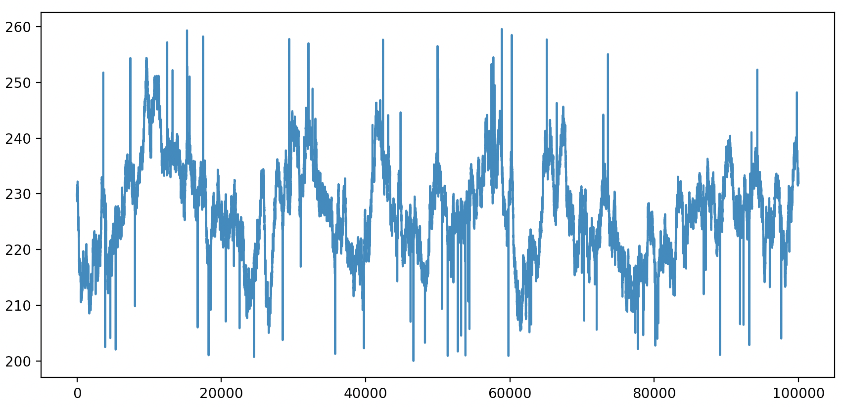
Let’s explain what this means. We take the normal voltage output of a european socket:

• key: the column/sub-column/field name where the value will be written

• type: the type of sensor to use (currently FLOAT and BOOL are supported)

• mean: the average output is 230V

• min/max: the voltage can change between ± 30V. So min is 200V and max is 260V

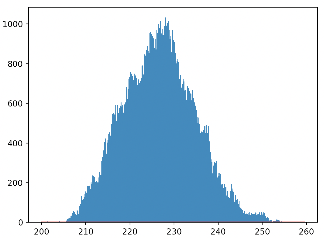
• stdev: we set the stdev to 10 so most values will be between 220V and 240V

• variance: limits the step size between values. In this example the value changes at most by 0.03V

• error_rate: The sensor has a 1:1000 chance to malfunction and report wrong values

• error_length: When the sensor malfunctions and reports a wrong value on average the next 2.5 values are also wrong

Using this schema to generate 100.000 values, the curve will look something like this (the spikes are the errors):

The value distribution of this curve will look something like this:

Boolean Sensor

The boolean sensor produces boolean values according to a given ratio. The schema for a boolean sensor is pretty simple, see also Data Generator Schema.

{
  "button_press": {
    "key": {
      "value": "button_pressed"
    },
    "type": {
      "value": "BOOL"
    },
    "true_ratio": {
      "value": 0.001
    }
  }
}

key:

The column/sub-column/field name where the value will be written.

type:

The type of sensor to use. Currently, FLOAT and BOOL are supported.

true_ratio:

The ratio how many time the Bool Sensor will generate the value True. E.g. if value is 1, the sensor will output True every time. If the value is 0.5, the output will be 50% True and 50% False.

Complex Schema Example

Use Case

We want to describe channels for:

• We have 50 plants

• Each plant contains of 5 lines

• Each line consists of 10 machines

• Each machine has 5 different sensors:

  • voltage

  • current

  • temperature

  • power

  • vibration

Solution

The first thing we need to identify how many channels we have in total: 50 plants * 5 lines * 10 machines = 2500 channels total. Now we know that we have to use 2500 IDs so we set ID_START=1 and ID_END=2500. Then we create our schema:

{
  "example": {
    "tags": {
      "plant": 50,
      "line": 5,
      "machine": "id"
    },
    "fields": {
      "voltage": {"..."},
      "current": {"..."},
      "temperature": {"..."},
      "power": {"..."},
      "vibration": {"..."}
    }
  }
}

As you see even a complex schema isn’t that complicated to write. The main limitation of the Data Generator is that one instance can only take a single schema. But when combining multiple instances it is easily possible to simulate complex setups spanning multiple factories with multiple machinery.

Batch Size Automator

To optimize ingest performance, the Batch Size Automator utility library is used. The BSA is only active when INGEST_MODE is set to 1, and BATCH_SIZE has a value smaller or equal 0. When activated, everything else is configured automatically.

Prometheus Metrics

An overview over the available Prometheus metrics and what they represent.

Query Timer Statistics Arguments

Metric Name	Description
tsperf_generated_values	How many values have been generated
tsperf_inserted_values	How many values have been inserted
tsperf_insert_percentage	INGEST_SIZE times number of IDs divided by number of inserted values
tsperf_batch_size	The currently used batch size [1]
tsperf_insert_time	The average time it took to insert the current batch into the database [1]
tsperf_rows_per_second	The average number of rows per second with the latest batch size [1]
tsperf_best_batch_size	The best batch size found by the batch size automator up to now [1]
tsperf_best_batch_rps	The rows per second number for the best batch size up to now [1]
tsperf_values_queue_was_empty	How many times the internal queue was empty when the insert threads requested values. This can indicate whether data generation lacks behind data insertion.
tsperf_inserts_failed	How many times the insert operation has failed
tsperf_inserts_performed_success	How many times the insert operation was performed successfully. For databases where a single insert operation has to be split into multiple ones. For AWS Timestream, still only one is counted.

Example Use Cases

This chapter gives examples on how the Data Generator can be used. The respective files for the examples can be explored in the schema folder.

Single channel

We want to simulate two factories each with ten lines and each line with five sensors/channels.

The sensor measures three readings:

• speed (float) in m/s

• temperature (float) in °C

• vibration (bool) above or below threshold

Every 5 seconds each sensor reports a value and we want our simulation to run for one hour.

Setup

The resulting JSON schema could look like machine.json.

As we have five sensors on ten lines in two factories we have 100 sensors in total, so for our docker-compose file we set the following environment variables:

• ID_START: 1

• ID_END: 100

As we want to use CrateDB running on localhost, we set the following environment variables:

• ADAPTER: “cratedb”

• ADDRESS: “host.docker.internal:4200”

• USERNAME: “aValidUsername”

• PASSWORD: “PasswordForTheValidUsername”

Note

host.docker.internal:4200 is the correct database address when trying to access CrateDB running on localhost, from inside a Docker container.

As we want to have a consistent insert every 5 seconds for one hour we set the following environment variables:

• INGEST_MODE: 0

• INGEST_SIZE: 720 (an hour has 3600 seconds divided by 5 seconds)

• TIMESTAMP_DELTA: 5

Finally, we want to signal using the appropriate schema:

• SCHEMA: “tsperf.schema.factory.simple:machine.json”

The resulting yml file could look like this:

version: "2.3"
services:
  datagen:
    image: ghcr.io/crate/tsperf:latest
    ports:
      - 8000:8000
    environment:
      ID_START: 1
      ID_END: 100

      INGEST_MODE: 0
      INGEST_SIZE: 720
      TIMESTAMP_DELTA: 5

      ADAPTER: cratedb
      ADDRESS: "host.docker.internal:4200"
      #USERNAME: ""
      #PASSWORD: ""
      SCHEMA: "tsperf.schema.factory.simple:machine.json"

Usage

To run this example follow the following steps:

• Start an instance of CrateDB on localhost.

  docker run --rm -it --publish="4200:4200" crate
  

• Enter USERNAME and PASSWORD in the simple factory compose file.

  • If no user was created, you can just delete both environment variables. CrateDB will use a default user.

• Start TSPERF using Docker Compose.

  docker-compose -f examples/factory-simple-machine.yml up
  

You can now navigate to localhost:4200 to look at CrateDB or to localhost:8000 to look at the raw data of the Data Generator.

Multiple channels

Note the provided examples for this use-case are supposed to run with CrateDB. To run it with other Databases changes according to the documentation have to be made. This use-case is not possible to run with TimescaleDB as it uses a fixed schema and adding columns to existing tables is not yet supported.

We want to simulate ten factories in ten different countries (defined by country code in the tag value) with ten lines per factory. The lines are grouped into upper lines and lower lines, with five lines per group. The different combinations have multiple sensors reporting at different time intervals:

• All lines in all factories have five sensors reporting a speed and vibration metric each second.

• All lines in the factories ["AT", "BE", "CH", "DE", "ES"] have five sensors reporting a voltage and current metric each second.

• All lines in all factories have two sensors reporting a temperature metric every ten seconds. The temperature values are different depending on which group the lines are in.

Setup

As we actually use four different schemas (temperature metric is different for upper and lower lines) we also have four different schema files. You can find them in the complex factory schemas folders.

To run this use-case we have to write a more complex docker-compose complex factory compose file.

Note we use INGEST_MODE: 1 to insert data fast. To keep data-size small we only insert 1000 seconds worth of data, this can obviously be adjusted to create a bigger dataset.

Usage

To run this example follow the following steps:

• Start an instance of CrateDB on localhost.

  docker run --rm -it --publish="4200:4200" crate
  

• Adjust USERNAME and PASSWORD in the complex factory compose file.

  • If no user was created, you can just ignore both environment variables. CrateDB will use a default user.

• Start TSPERF using Docker Compose.

  docker-compose -f examples/factory-complex-scenario.yml up
  

You can now navigate to http://localhost:4200/ to look at CrateDB, or to http://localhost:8000/ to look at the raw data of the Data Generator.

Glossary

• Sensor: A “sensor” yields a single reading/value.

• Channel: A “channel” is a container for measurements of multiple sensors.

• Plant:

• Line:

• Machine:

---

[1] (1,2,3,4,5)

Only available with Batch Size Automator.